Sparsity with MirrorCBO

Imports

We need numpy and the CBXPy package.

• MirrorCBO is the main class for the Mirror CBO algorithm.

• ElasticNet is a specific mirror map that we will use in this example.

• scheduler is used to adjust parameters during optimization.

from cbx.dynamics.mirrorcbo import MirrorCBO, ElasticNet
from cbx.scheduler import multiply
import numpy as np
import matplotlib.pyplot as plt

Create a synthetic optimization problem

We consider sparse signal recovery. We create a random matrix A and a sparse vector x0, and we observe b = A x0 + noise. The goal is to recover x0 from A and b. The loss function is the least squares loss.

dim = 30
num_signals = 3
sigma = 0.01
A = np.random.randn(dim, dim)
x_true = np.zeros(dim)
idx    = np.random.permutation(dim)[:num_signals]
x_true[idx] = np.random.randn(num_signals)
meas = A @ x_true + sigma * np.random.randn(dim)

def loss(x):
    return 0.5 * np.linalg.norm(x @ A.T - meas, axis=-1)**2

Run the Mirror CBO algorithm

We create an instance of the MirrorCBO class with the specified parameters, including the mirror map, noise type, and time step. We then call the optimize method to run the optimization process. We use a scheduler to adjust parameters during optimization.

Note: CBO performance is sensitive. Finetuning for different problems might be necessary.

dyn = MirrorCBO(loss, N= 100, d = dim, mirrormap=ElasticNet(1.9),
                noise = 'anisotropic', sigma = 2.,
                dt = 0.05,
                max_it=100)
sched = multiply(factor = 1.4)
dyn.optimize(sched=sched, print_int = 20)
x = dyn.best_particle[0,:]

....................
Starting Optimization with dynamic: MirrorCBO
....................
Time: 1.000, best current energy: [7.13625709]
Number of function evaluations: [2100]
Time: 2.000, best current energy: [0.00419865]
Number of function evaluations: [4100]
Time: 3.000, best current energy: [0.00219423]
Number of function evaluations: [6100]
Time: 4.000, best current energy: [0.00219431]
Number of function evaluations: [8100]
Time: 5.000, best current energy: [0.0021943]
Number of function evaluations: [10100]
--------------------
Finished solver.
Best energy: [0.00219412]
--------------------

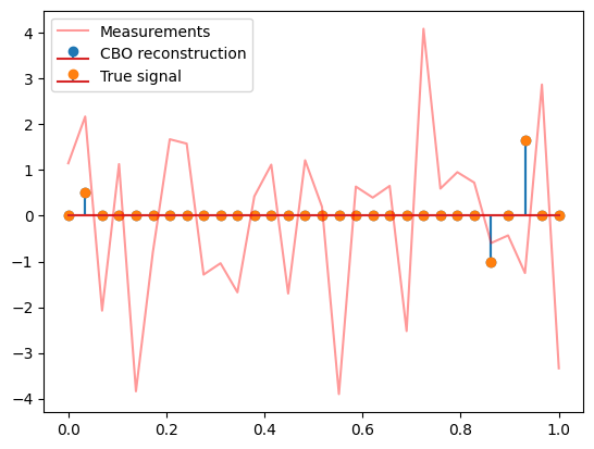
Plot results

s = np.linspace(0,1, dim)
plt.stem(s, x, '-o', label='CBO reconstruction')
plt.stem(s, x_true, '-o', label='True signal')
plt.plot(s, meas, color='r', alpha=0.4, label='Measurements')
plt.legend()

<matplotlib.legend.Legend at 0x22290258500>